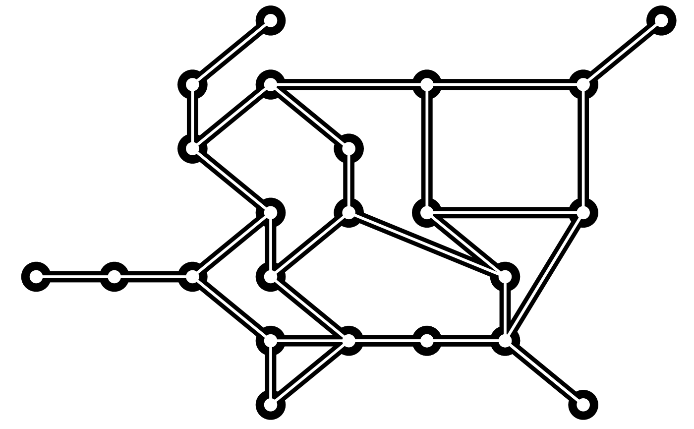
In very short terms, a layout is the vertical and horizontal
placement of nodes when plotting a particular graph structure.
Conversely, a layout algorithm is an algorithm that takes in a graph
structure (and potentially some additional parameters) and return the
vertical and horizontal position of the nodes. Often, when people think
of network visualizations, they think of node-edge diagrams where
strongly connected nodes are attempted to be plotted in close proximity.
Layouts can be a lot of other things too though — e.g. hive plots and
treemaps. One of the driving factors behind ggraph has been
to develop an API where any type of visual representation of graph
structures is supported. In order to achieve this we first need a
flexible way of defining the layout…
The ggraph() and create_layout() functions
As the layout is a global specification of the spatial position of
the nodes it spans all layers in the plot and should thus be defined
outside of calls to geoms or stats. In ggraph it is often
done as part of the plot initialization using ggraph() — a
function equivalent in intent to ggplot(). As a minimum
ggraph() must be passed a graph object supported by
ggraph:
library(ggraph)
library(tidygraph)

set_graph_style(plot_margin = margin(1,1,1,1))
graph <- as_tbl_graph(highschool)

# Not specifying the layout - defaults to "auto"
ggraph(graph) +
  geom_edge_link(aes(colour = factor(year))) +
  geom_node_point()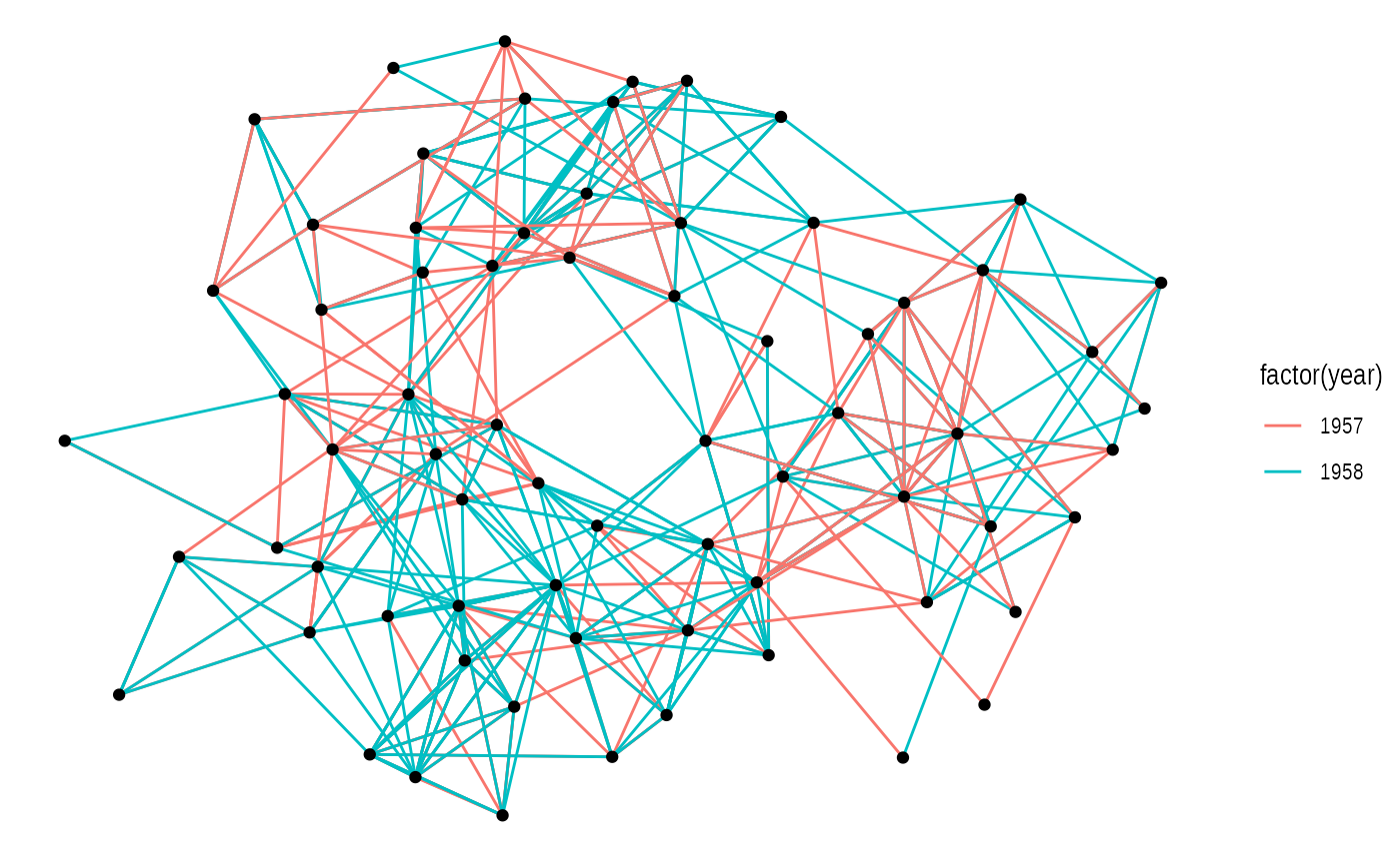
Not specifying a layout will make ggraph pick one for
you. This is only intended to get quickly up and running. The choice of
layout should be deliberate on the part of the user as it will have a
great effect on what the end result will communicate. From now on all
calls to ggraph() will contain a specification of the
layout:
ggraph(graph, layout = 'kk') +
  geom_edge_link(aes(colour = factor(year))) +
  geom_node_point()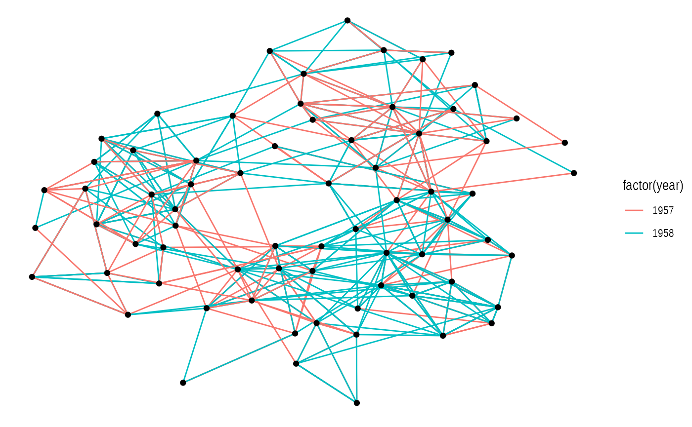
If the layout algorithm accepts additional parameters (most do), they
can be supplied in the call to ggraph() as well:
ggraph(graph, layout = 'kk', maxiter = 100) +
  geom_edge_link(aes(colour = factor(year))) +
  geom_node_point()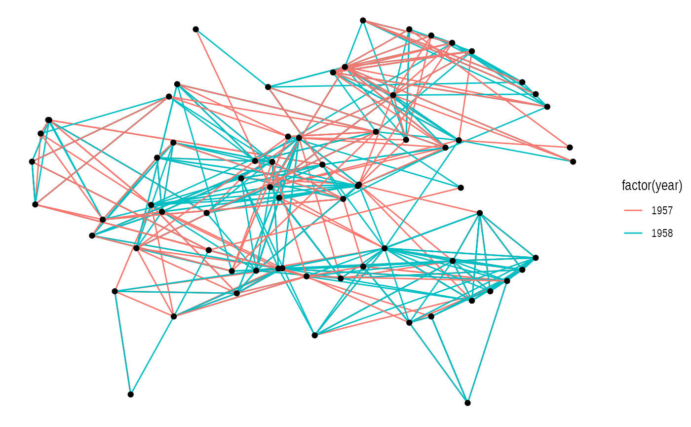
If any layout parameters refers to node or edge variables they must
be supplied as unquoted expression (like inside aes() and
tidyverse verbs)
In addition to specifying the layout during plot creation it can also
happen separately using create_layout(). This function
takes the same arguments as ggraph() but returns a
layout_ggraph object that can later be used in place of a
graph structure in ggraph call:
layout <- create_layout(graph, layout = 'eigen')## Warning in layout_with_eigen(graph, type = type, ev = eigenvector): g is
## directed. undirected version is used for the layout.
ggraph(layout) +
  geom_edge_link(aes(colour = factor(year))) +
  geom_node_point()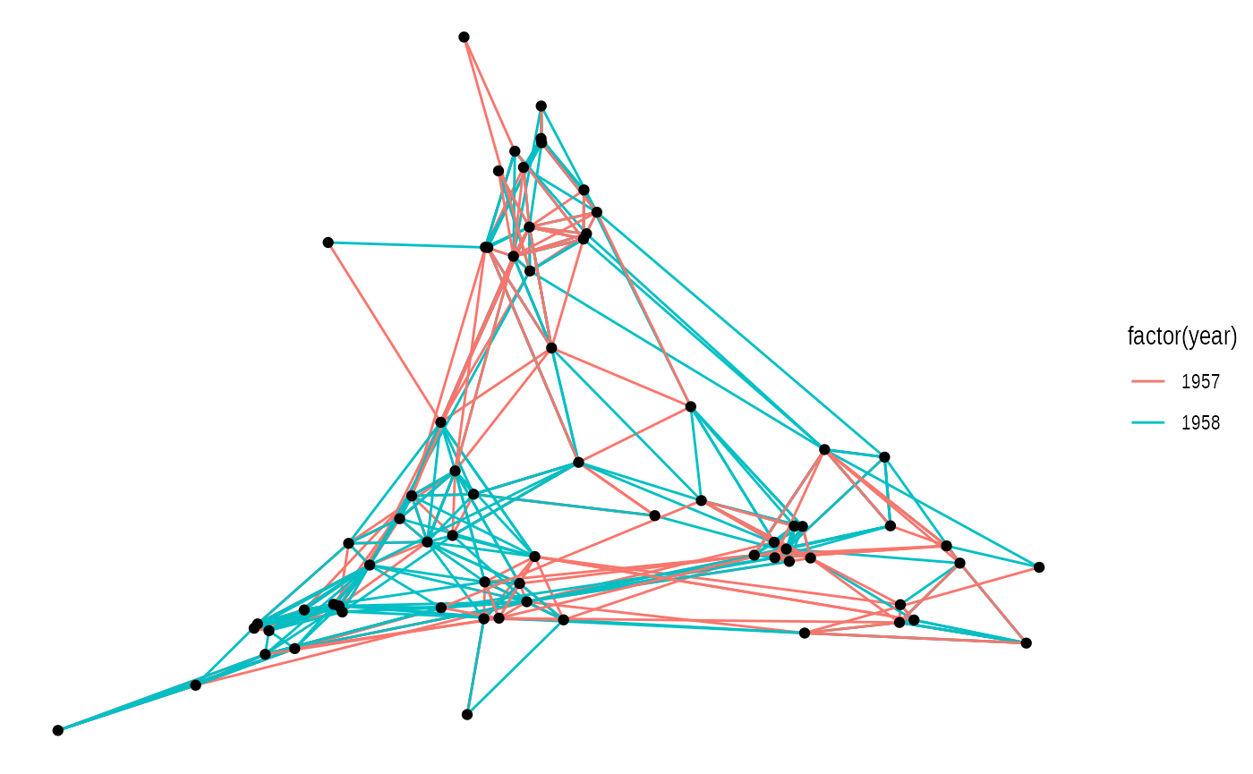
Examining the return of create_layout() we see that it
is really just a data.frame of node positions and
(possible) attributes. Furthermore the original graph object along with
other relevant information is passed along as attributes:
head(layout)## # A tibble: 6 × 5
## x y circular .ggraph.orig_index .ggraph.index
## <dbl> <dbl> <lgl> <int> <int>
## 1 -0.0447 0.156 FALSE 1 1
## 2 -0.0374 0.208 FALSE 2 2
## 3 -0.0565 0.299 FALSE 3 3
## 4 0.180 -0.0348 FALSE 4 4
## 5 0.177 0.0122 FALSE 5 5
## 6 0.00998 0.195 FALSE 6 6
attributes(layout)## $names
## [1] "x" "y" "circular"
## [4] ".ggraph.orig_index" ".ggraph.index"
##
## $row.names
## [1] 1 2 3 4 5 6 7 8 9 10 11 12 13 14 15 16 17 18 19 20 21 22 23 24 25
## [26] 26 27 28 29 30 31 32 33 34 35 36 37 38 39 40 41 42 43 44 45 46 47 48 49 50
## [51] 51 52 53 54 55 56 57 58 59 60 61 62 63 64 65 66 67 68 69 70
##
## $class
## [1] "layout_tbl_graph" "layout_ggraph" "tbl_df" "tbl"
## [5] "data.frame"
##
## $graph
## # A tbl_graph: 70 nodes and 506 edges
## #
## # A directed multigraph with 1 component
## #
## # Node Data: 70 × 3 (active)
## .ggraph.orig_index .ggraph_layout_x .ggraph_layout_y
## <int> <dbl> <dbl>
## 1 1 -0.0447 0.156
## 2 2 -0.0374 0.208
## 3 3 -0.0565 0.299
## 4 4 0.180 -0.0348
## 5 5 0.177 0.0122
## 6 6 0.00998 0.195
## 7 7 -0.0137 0.252
## 8 8 -0.0138 0.230
## 9 9 -0.0200 0.139
## 10 10 0.104 -0.0548
## # ℹ 60 more rows
## #
## # Edge Data: 506 × 3
## from to year
## <int> <int> <dbl>
## 1 1 13 1957
## 2 1 14 1957
## 3 1 20 1957
## # ℹ 503 more rows
##
## $circular
## [1] FALSEAs it is just a data.frame it means that any standard
ggplot2 call will work by addressing the nodes. Still, use
of the geom_node_*() family provided by ggraph
is encouraged as it makes it explicit which part of the data structure
is being worked with.
Adding support for new data sources
Out of the box ggraph supports tbl_graph
objects from tidygraph natively. Any other type of object will be
attempted to be coerced to a tbl_graph object
automatically. Tidygraph provide conversions for most known graph
structure in R so almost any data type is supported by ggraph by
extension. If there is wish for support for additional classes this can
be achieved by providing a as_tbl_graph() method for the
class. If you do this, consider submitting the method to tidygraph so
others can benefit from your work.
Layouts abound
There’s a lot of different layouts in ggraph — All
layouts from the graphlayouts and igraph packages are available, and
ggraph itself also provides some of the more specialised layouts itself.
All in all, ggraph provides well above 20 different layouts to choose
from, far more than we can cover in this text. I urge you to explore the
different layout types. Blindly running along with the default layouts
is a sad but common mistake in network visualisation that can cloud or
distort the insight the network might hold. If ggraph lacks the needed
layout it is always possible to supply your own layout function that
takes a tbl_graph object and returns a data.frame of node positions, or
supply the positions directly by passing a matrix or data.frame to the
layout argument.
A note on circularity
Some layouts can be shown effectively both in a standard Cartesian
projection as well as in a polar projection. The standard approach in
ggplot2 has been to change the coordinate system with the
addition of e.g. coord_polar(). This approach — while
consistent with the grammar — is not optimal for ggraph as
it does not allow layers to decide how to respond to circularity. The
prime example of this is trying to draw straight lines in a plot using
coord_polar(). Instead circularity is part of the layout
specification and gets communicated to the layers with the
circular column in the data, allowing each layer to respond
appropriately. Sometimes standard and circular representations of the
same layout get used so often that they get different names. In
ggraph they’ll have the same name and only differ in
whether or not circular is set to TRUE:
# An arc diagram
ggraph(graph, layout = 'linear') +
  geom_edge_arc(aes(colour = factor(year)))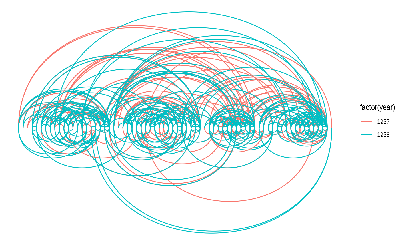
# A coord diagram
ggraph(graph, layout = 'linear', circular = TRUE) +
  geom_edge_arc(aes(colour = factor(year))) +
  coord_fixed()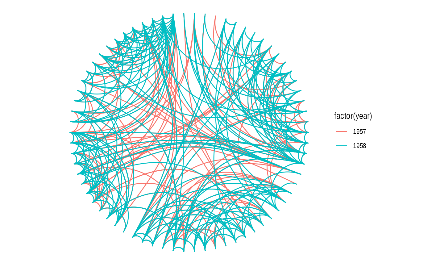
graph <- tbl_graph(flare$vertices, flare$edges)
# An icicle plot
ggraph(graph, 'partition') +
  geom_node_tile(aes(fill = depth), size = 0.25)
## Warning: Using `size` aesthetic for lines was deprecated in ggplot2 3.4.0.
## ℹ Please use `linewidth` instead.
## This warning is displayed once every 8 hours.
## Call `lifecycle::last_lifecycle_warnings()` to see where this warning was
## generated.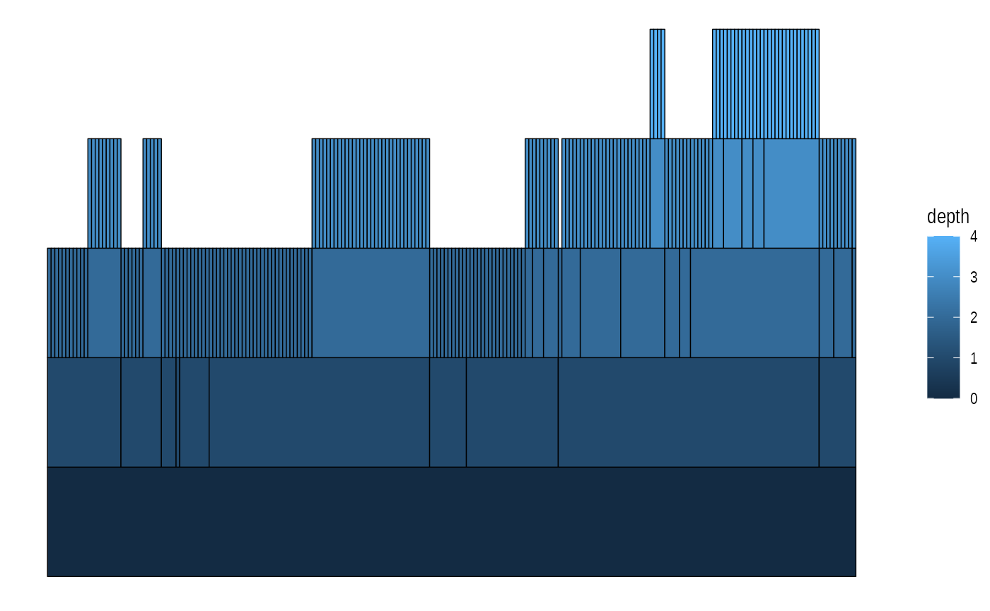
# A sunburst plot
ggraph(graph, 'partition', circular = TRUE) +
  geom_node_arc_bar(aes(fill = depth), size = 0.25) +
  coord_fixed()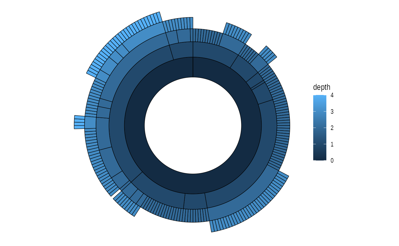
Not every layout has a meaningful circular representation in which
cases the circular argument will be ignored.
Node-edge diagram layouts
Both graphlayout and igraph provides a
range of different layout algorithms for classic node-edge diagrams
(colloquially referred to as hairballs). Some of these are incredibly
simple such as randomly, grid, circle, and
star, while others tries to optimize the position of nodes
based on different characteristics of the graph. There is no such thing
as “the best layout algorithm” as algorithms have been optimized for
different scenarios. Experiment with the choices at hand and remember to
take the end result with a grain of salt, as it is just one of a range
of possible “optimal node position” results. Below is a sample of some
of the layouts available through igraph applied to the
highschool graph.
graph <- as_tbl_graph(highschool) |>
  mutate(degree = centrality_degree())
lapply(c('stress', 'fr', 'lgl', 'graphopt'), function(layout) {
  ggraph(graph, layout = layout) +
    geom_edge_link(aes(colour = factor(year)), show.legend = FALSE) +
    geom_node_point() +
    labs(caption = paste0('Layout: ', layout))
})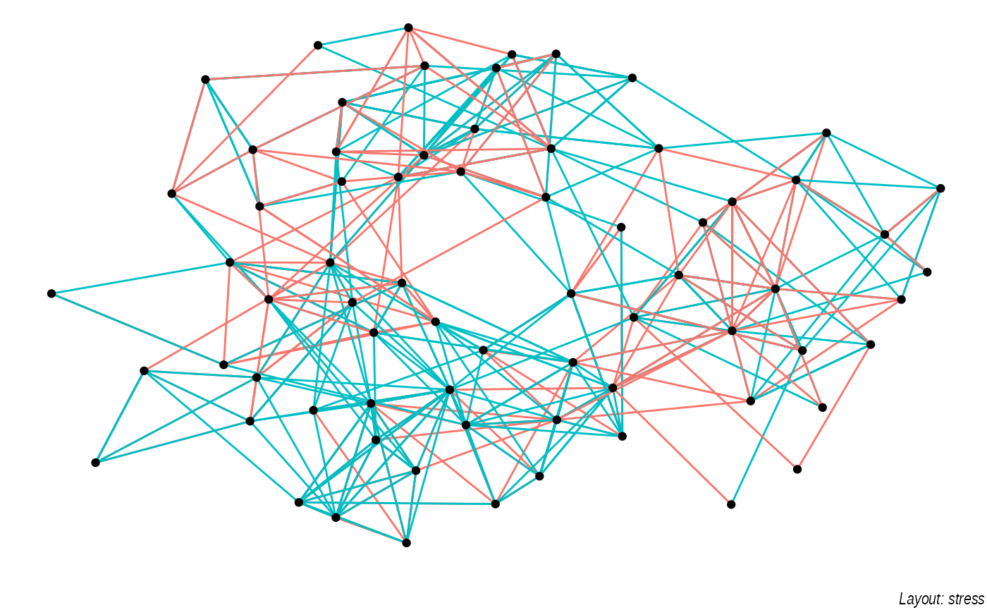
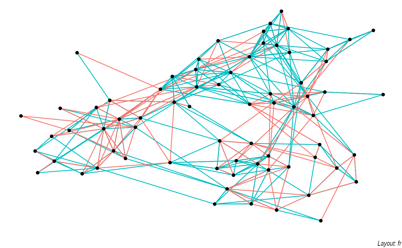
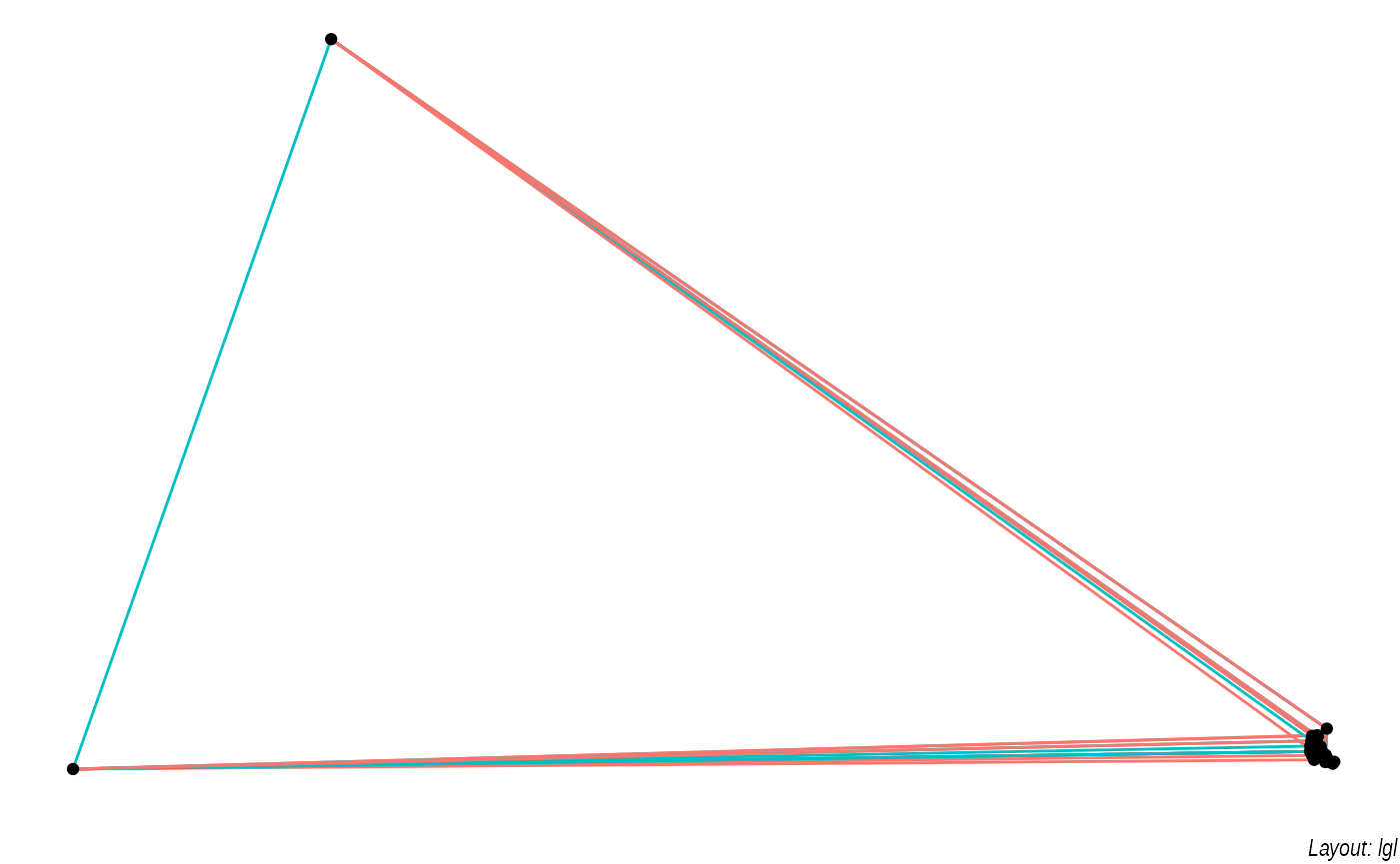
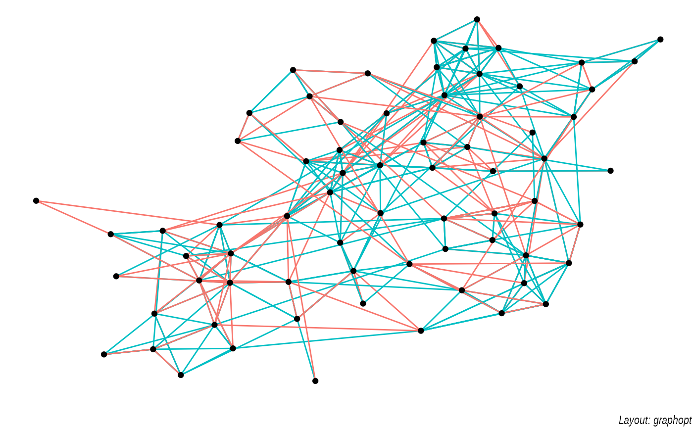
The default plot is the "stress" layout that uses stress
majorization to spread out nodes. It generally does a good job and is
deterministic so that it doesn’t change upon every call (many other
layouts does that as they use randomisation for the initial node
positions). The stress layout also makes it possible to fix the location
of certain nodes in one or two dimensions making it a very versatile
starting point for your visualisation.
Hive plots
A hive plot, while still technically a node-edge diagram, is a bit different from the rest as it uses information pertaining to the nodes, rather than the connection information in the graph. This means that hive plots, to a certain extent are more interpretable as well as less vulnerable to small changes in the graph structure. They are less common though, so use will often require some additional explanation.
graph <- graph |>
  mutate(friends = ifelse(
    centrality_degree(mode = 'in') < 5, 'few',
    ifelse(centrality_degree(mode = 'in') >= 15, 'many', 'medium')
  ))
ggraph(graph, 'hive', axis = friends, sort.by = degree) +
  geom_edge_hive(aes(colour = factor(year))) +
  geom_axis_hive(aes(colour = friends), size = 2, label = FALSE) +
  coord_fixed()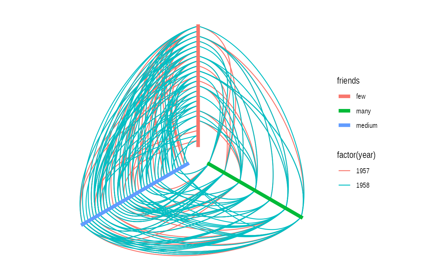
Focal layouts
Some layouts can put focus on a single node or a group of nodes by
defining all other positions relative to that. An example of this is the
focus layout, but the centrality layout is
very akin to it:
ggraph(graph, 'focus', focus = node_is_center()) +
  ggforce::geom_circle(aes(x0 = 0, y0 = 0, r = r), data.frame(r = 1:5), colour = 'grey') +
  geom_edge_link() +
  geom_node_point() +
  coord_fixed()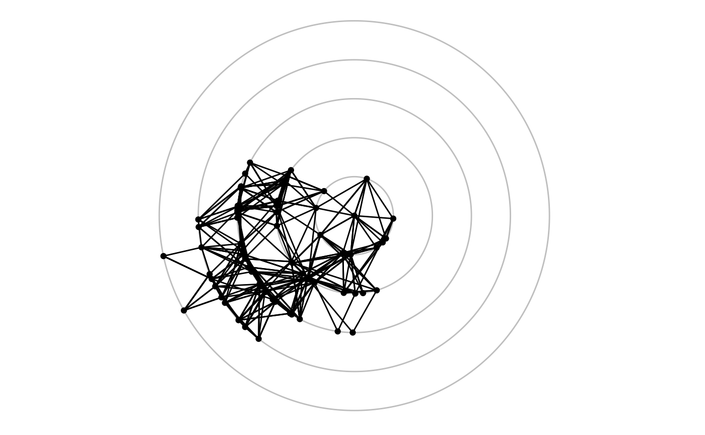
Hierarchical layouts
Trees and hierarchies are an important subset of graph structures,
and ggraph provides a range of layouts optimized for their
visual representation. Some of these use enclosure and position rather
than edges to communicate relations (e.g. treemaps and circle packing).
Still, these layouts can just as well be used for drawing edges if you
wish to:
graph <- tbl_graph(flare$vertices, flare$edges)
set.seed(1)
ggraph(graph, 'circlepack', weight = size) +
  geom_node_circle(aes(fill = depth), size = 0.25, n = 50) +
  coord_fixed()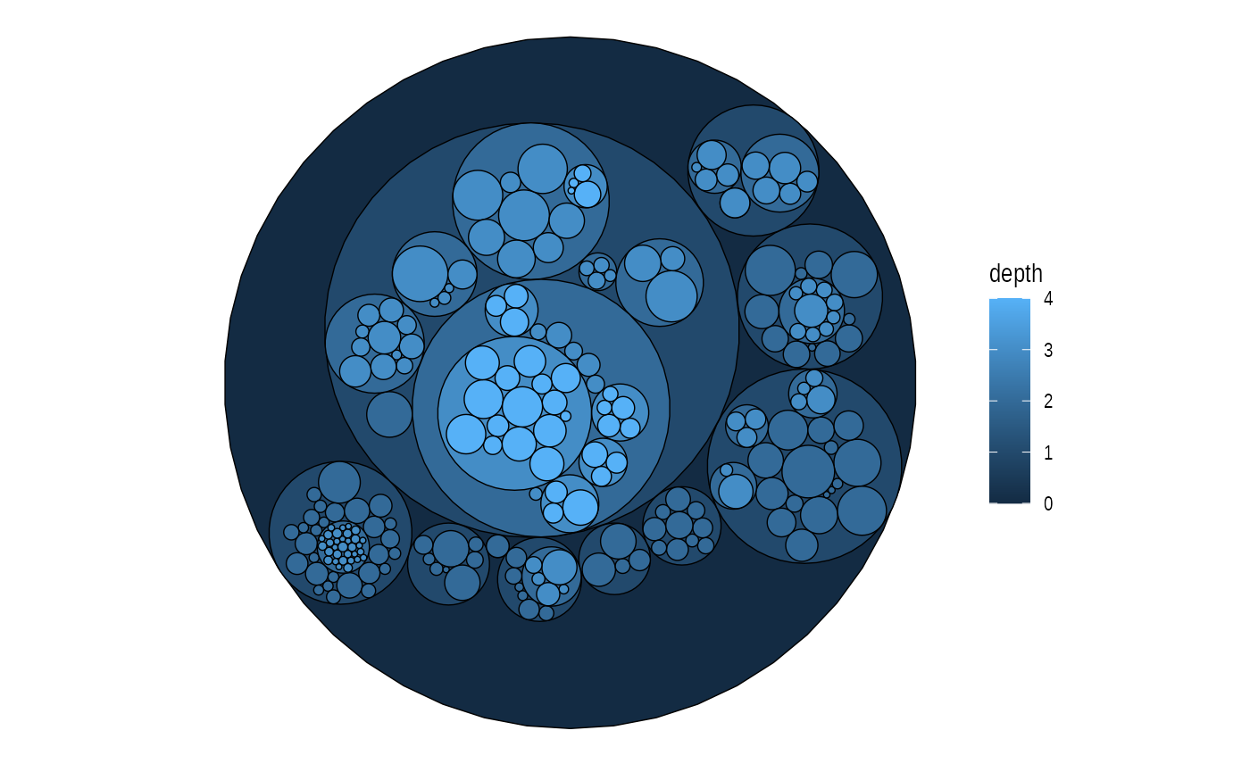
set.seed(1)
ggraph(graph, 'circlepack', weight = size) +
  geom_edge_link() +
  geom_node_point(aes(colour = depth)) +
  coord_fixed()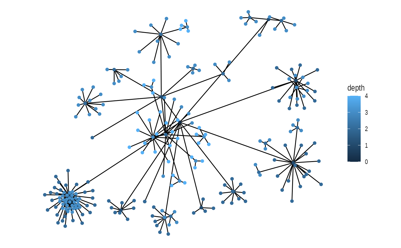
ggraph(graph, 'treemap', weight = size) +
  geom_node_tile(aes(fill = depth), size = 0.25)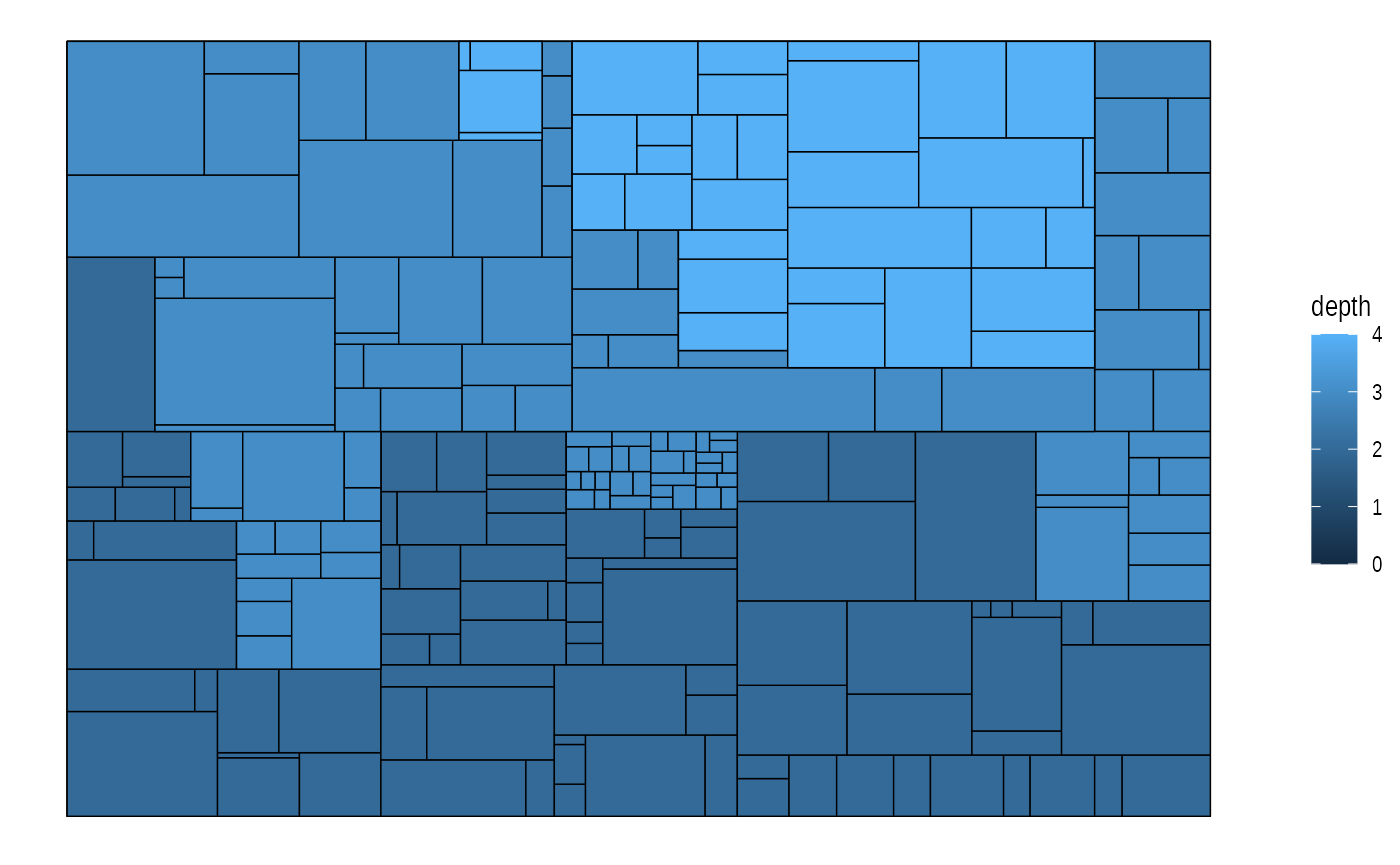
ggraph(graph, 'treemap', weight = size) +
  geom_edge_link() +
  geom_node_point(aes(colour = depth))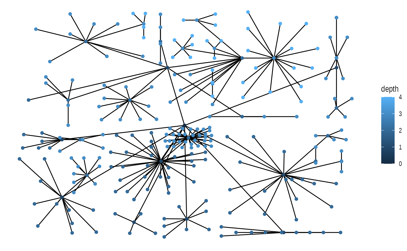
Cactustree is a layout type specifically developed for use with hierarchical edge bundling, but can be used on it’s own as well
ggraph(graph, 'cactustree') +
  geom_node_circle(aes(fill = depth), size = 0.25) +
  coord_fixed()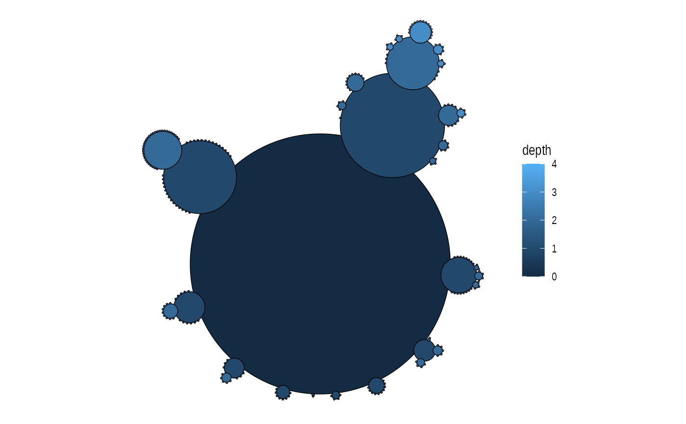
importFrom <- match(flare$imports$from, flare$vertices$name)
importTo <- match(flare$imports$to, flare$vertices$name)

ggraph(graph, 'cactustree') +
  geom_node_circle(aes(fill = depth),
    size = 0.25,
    alpha = 0.2
  ) +
  geom_conn_bundle(aes(colour = after_stat(index)),
    data = get_con(importFrom, importTo),
    edge_alpha = 0.25
  ) +
  theme(legend.position = "none") +
  coord_fixed()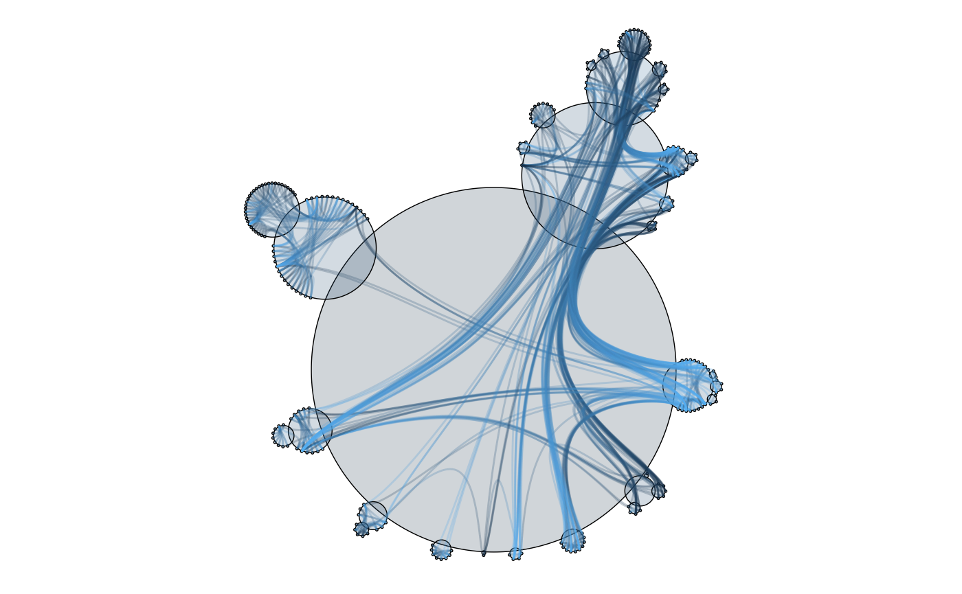
The most recognized tree plot is probably dendrograms though. If nothing else is stated the height of each node is calculated based on the distance to its farthest sibling (the tree layout, on the other hand, puts all nodes at a certain depth at the same level):
ggraph(graph, 'tree') +
  geom_edge_diagonal()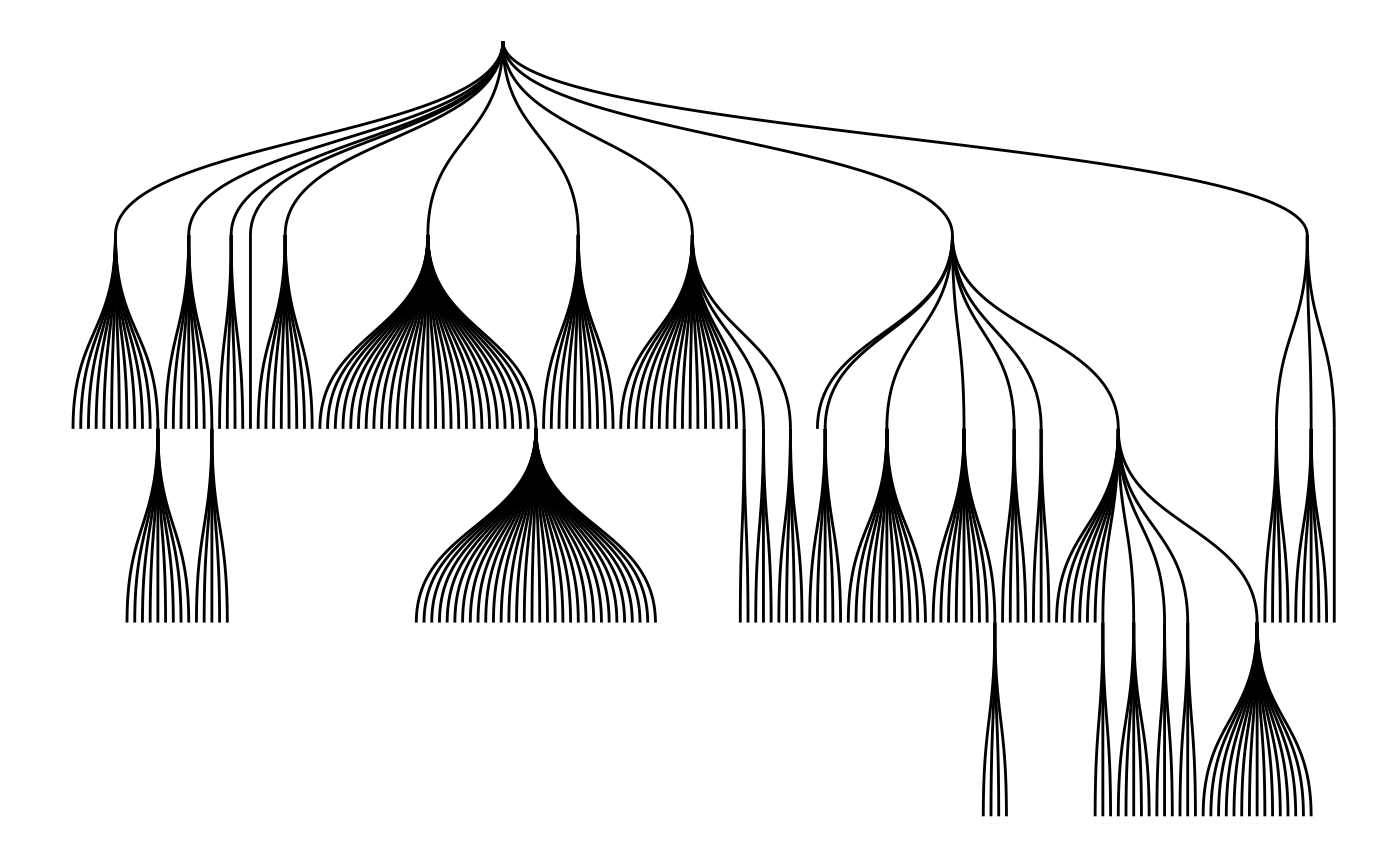
The height of each branch point can be set to a variable — e.g. the height provided by hclust and dendrogram objects:
dendrogram <- hclust(dist(iris[, 1:4]))
ggraph(dendrogram, 'dendrogram', height = height) +
  geom_edge_elbow()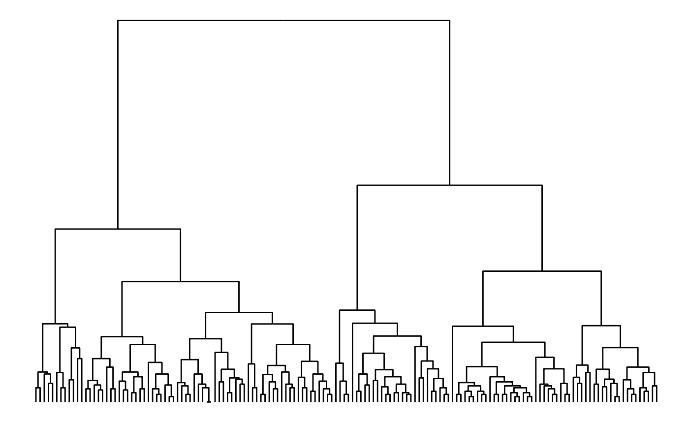
Dendrograms are one of the layouts that are amenable for circular transformations, which can be effective in giving more space at the leafs of the tree at the expense of the space given to the root:
ggraph(dendrogram, 'dendrogram', circular = TRUE) +
  geom_edge_elbow() +
  coord_fixed()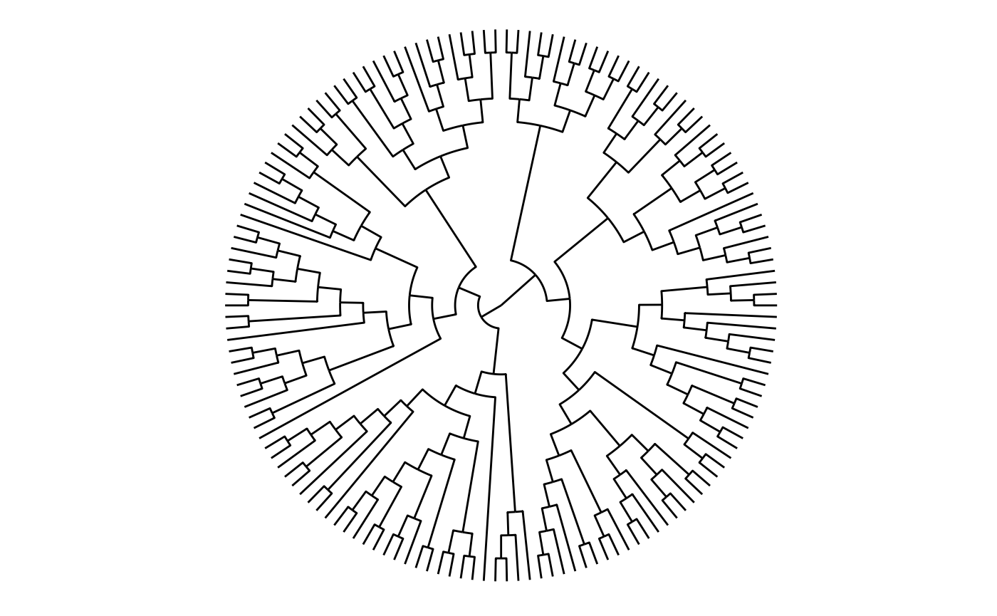
A type of trees known especially in phylogeny is unrooted trees,
where no node is considered the root. Often a dendrogram layout will not
be faithful as it implicitly position a node at the root. To avoid that
you can use the unrooted layout instead.
tree <- create_tree(100, 2, directed = FALSE) |>
  activate(edges) |>
  mutate(length = runif(n()))
ggraph(tree, 'unrooted', length = length) +
  geom_edge_link()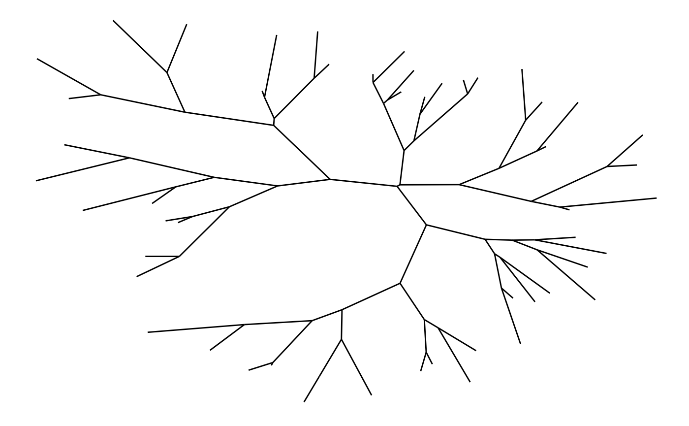
Often unrooted trees have a branch length attached - this can be
passed to both the dendrogram and unrooted
layout to determine the length of each edge.
Matrix layouts
Many node-edge diagram layouts suffer from poor scalability, where edges will eventually begin to overlap to the extend that the plot becomes unintellible. One way to combat this is by only plotting subsets of the larger plot, but another approach is to choose a layout that avoids overlapping edges altogether. The matrix layout places each node on a diagonal and draws edges by drawing points or tiles at the intersection of the vertical and horizontal position of its terminal nodes. Using matrix layouts efficiently requires that you begin to recognise the specific patterns that different network topologies gives rise to. Further, it is important to recognise the large effect that the node order has on the look of the matrix layout:
graph <- create_notable('zachary')
ggraph(graph, 'matrix', sort.by = node_rank_leafsort()) +
  geom_edge_point(mirror = TRUE) +
  coord_fixed()
## Warning in .hclust_helper(x, control): control parameter method is deprecated.
## Use linkage instead!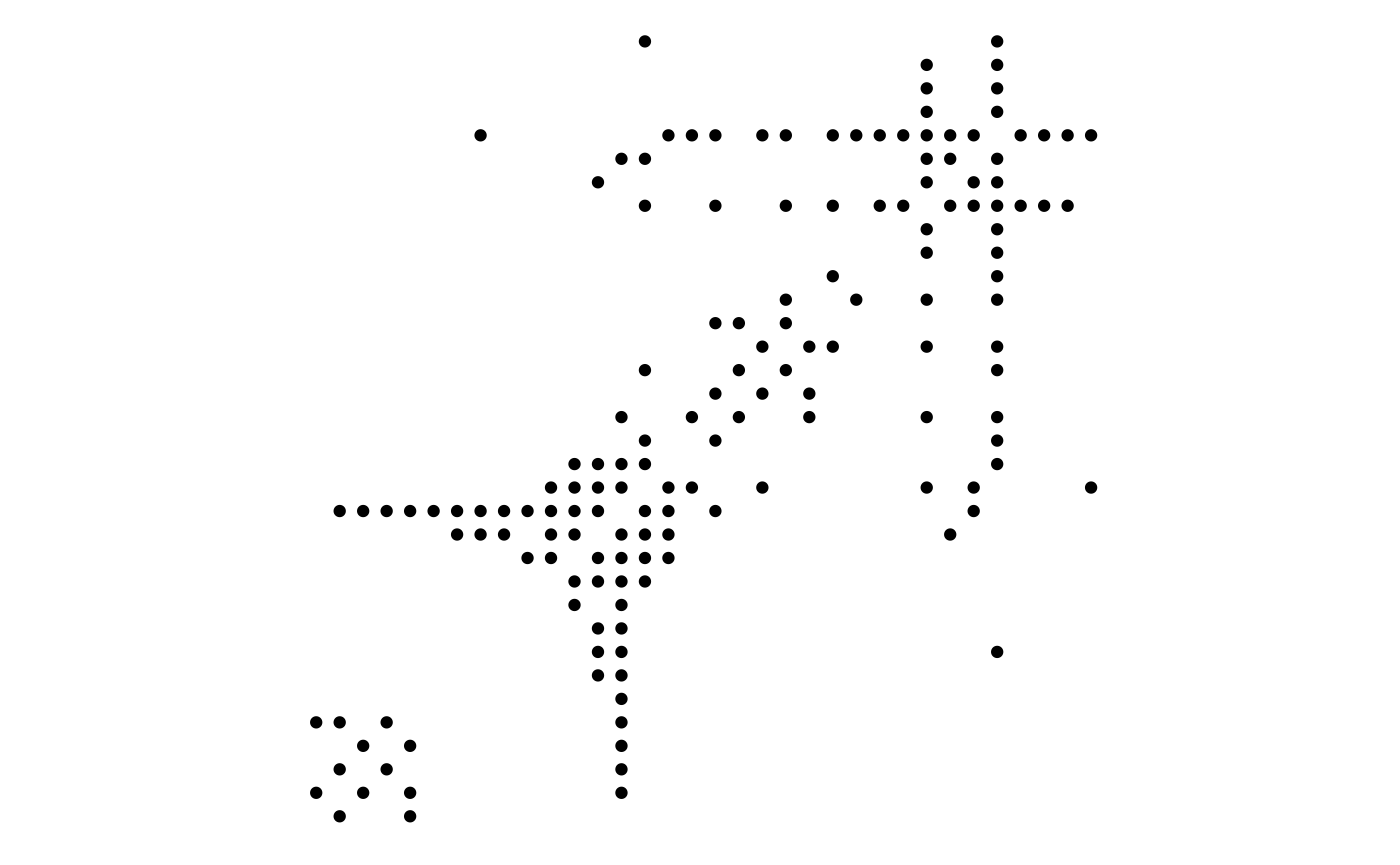
ggraph(graph, 'matrix', sort.by = node_rank_spectral()) +
  geom_edge_point(mirror = TRUE) +
  coord_fixed()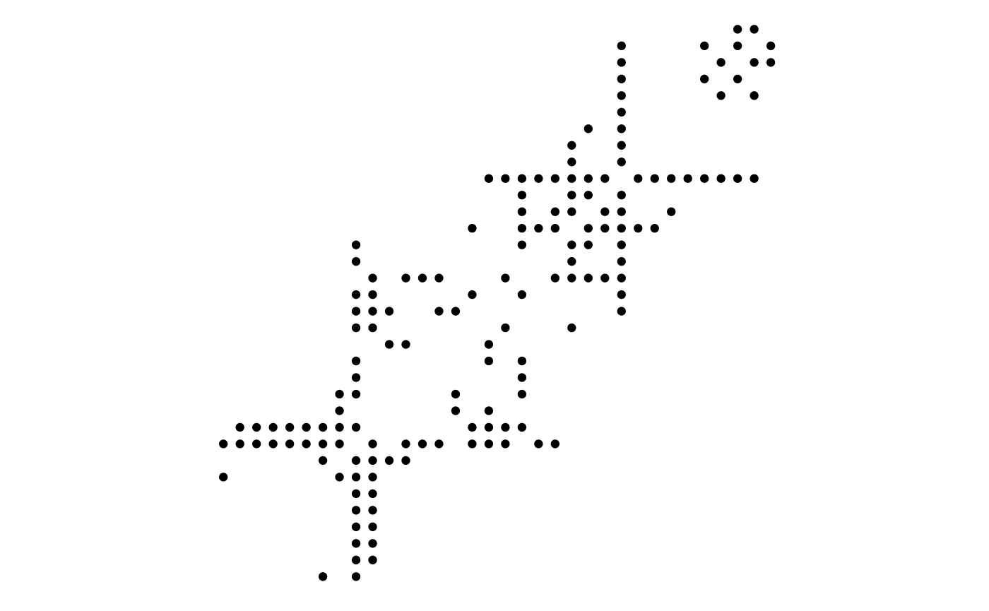
Fabric layouts
Another special layout that promises scalability is the biofabric
layout (here named fabric to avoid it being ignored for
non-biological networks). The fabric layout is special in that it
positions nodes evenly spaced on the y-axis and then draws edges as
vertical (and by extension, parallel) lines evenly separated as well,
connecting the nodes. Nodes are drawn as horizontal lines spanning the
extent of the edges that departs from it. As with matrix layouts the
node ordering have a huge impact on the final look and interpreting the
plot may take some getting used to.
ggraph(graph, 'fabric', sort.by = node_rank_fabric()) +
  geom_node_range(colour = 'grey') +
  geom_edge_span(end_shape = 'square') +
  coord_fixed()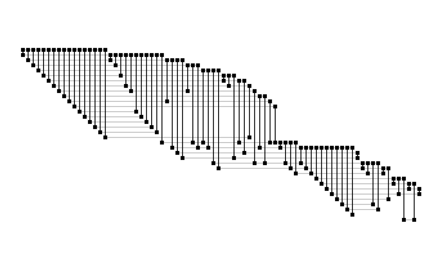
Fabric layouts allow something called shadow edges where all edges are duplicated to make it easier to follow all edges originating from each node.
ggraph(graph, 'fabric', sort.by = node_rank_fabric(), shadow.edges =TRUE) +
  geom_node_range(colour = 'grey') +
  geom_edge_span(aes(filter = shadow_edge), colour ='lightblue' , end_shape = 'square') +
  geom_edge_span(aes(filter = !shadow_edge), end_shape = 'square') +
  coord_fixed()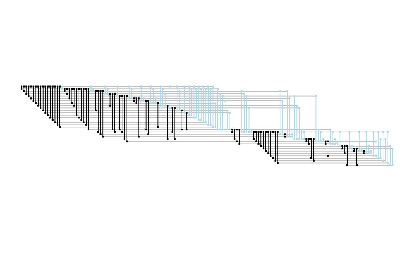
Spatial layouts
ggraph has a few layouts aimed at data where the node has a physical location. You may think this requires no layout at all and to some extent you are correct.
ggraph supports spatial networks through the sfnetworks package and grabs the node position and CRS from the data correctly when using the “sf” layout:
gr <- sfnetworks::as_sfnetwork(sfnetworks::roxel)## Registered S3 methods overwritten by 'proxy':
## method from
## print.registry_field registry
## print.registry_entry registry
ggraph(gr, 'sf') +
  geom_edge_sf(aes(color = type)) +
  geom_node_sf(size = 0.3)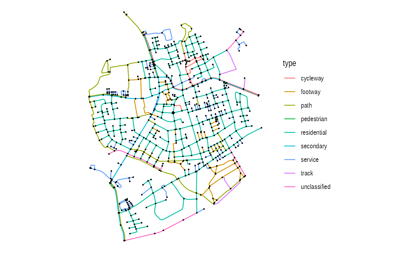
Another type of spatial layout is the metro layout which takes in a prior position and attempts to make these positions fit into a grid-like structure, well known in railroad and metro maps.
gr <- create_notable('Walther')
# Use stress layout to come up with a initial position
prior <- create_layout(gr, 'stress')

# Optimise placement with metro layout
ggraph(gr, 'metro', x = prior$x, y = prior$y, grid_space = 1, max_movement = 50) +
  geom_edge_link(width = 4) +
  geom_node_point(size = 10) +
  geom_edge_link(color = 'white', width = 1) +
  geom_node_point(color = 'white', size = 4)